Code
x <- c(1, 2, 4, 8, 16)
p <- c(0.4, 0.2, 0.2, 0.1, 0.1)

dis <- tibble(x=x,
              p=p)

dis %>%
    flextable()
x | p |
|---|---|
1 | 0.4 |
2 | 0.2 |
4 | 0.2 |
8 | 0.1 |
16 | 0.1 |
Chapter 2 notes
Markov’s Inequality states the following:
\(P(X \geq a) \leq \frac{E(X)}{a}\)
The probability of some data point in the distribution X exceeding some threshold value \(a\) cannot exceed the average of the distribution divided by \(a\).
When all we know about a distribution is it’s mean, Markov’s Inequality sets an upper bound on the probability of observing a particular value of any data point in the distribution.
How might this look in practice?
Let \(X\) be a discrete random variable with values \(x_1, x_2, \ldots, x_n\) and probabilities \(p_1, p_2, \ldots, p_n\) where \(X \geq 0\).
x <- c(1, 2, 4, 8, 16)
p <- c(0.4, 0.2, 0.2, 0.1, 0.1)
dis <- tibble(x=x,
p=p)
dis %>%
flextable()x | p |
|---|---|
1 | 0.4 |
2 | 0.2 |
4 | 0.2 |
8 | 0.1 |
16 | 0.1 |
We get the expected value, or average, of the variable by summing over each value in the distribution times its weight.
\[E(X) = \sum_i x_i \cdot P(X = x_i)\] \(E(X)\) = \((1)(.4) + (2)(.2) + (4)(.2) + (8)(.1) + (16)(.1)\)
So \(E(X)\) = 4
EX <- sum(x * p)Now let’s establish some arbitrary threshold \(a\geq4\)
In this example, what is \(P(X\geq a)\leq\frac{E(X)}{a}\)?
\(P(X\geq4)\leq\frac{4}{4}\leq 1\)
An obvious case, because the data point is also the mean!
What if \(a\geq8\)?
\(P(X\geq8)\leq\frac{4}{8}\leq.5\)
For a distribution with mean four, only half of all values of the distribution may exceed eight. If more than half of values in the distribution exceeded eight, it would shift the mean!
\(a\geq16\)?
\(P(X\ge16)\leq\frac{4}{16}\leq.25\)
For a distribution of mean four, at most 25 percent of all data values may exceed 16. As soon as more than 25 percent of data values exceed four, it will shift the mean.
Let’s work out how we can derive Markov’s Inequality, and offer additional illustrations
Note how we computed \(E(X)\) as the sum of all values times their weight.
\[E(X) = \sum_i x_i \cdot P(X = x_i)\]
Let’s do that again, but this time grouping terms around our threshold \(a=4\).1
1 This is the Law of Total Expectation: \(E(X) = E(X|A)P(A) + E(X|A^c)P(A^c)\)
\[E[X] = \sum\limits_{x_i < a} x_i \cdot P(X = x_i) + \sum\limits_{x_i \geq a} x_i \cdot P(X = x_i)\] In the example we’re working with, that would be
\(E(X) = \Big[ (1)(.4) + (2)(.2) \Big] + \Big[ (4)(.2) + (8)(.1) + (16)(.1) \Big]\)
We’re only interested in the second part of the decomposition. What happens if we remove the first part where \(a\lt 4\)?
Since all values of \(X\) are non-negative, that means we are removing positive values from the sum. Because we are removing positive values from the sum, the result of the operation will be less than \(E(X)\). Therefore, \(E(X)\) will be the same as or higher than the remaining sum.
This allows us to replace the equality with greater than or equal to.
\[E(X) \geq \sum\limits_{x_i \geq a} x_i \cdot P(X = x_i)\]
Returning to our example, that would be
\(E(X) \geq (4)(.2) + (8)(.1) + (16)(.1)\)
Recall that \(E(X)=4\) and \(E(X\geq4)=.8 + .8 + 1.6 = 3.2\)
\(4\geq3.2\) and our inequality holds
Let’s go back to the generalized notation:
\[E(X) \geq \sum\limits_{x_i \geq a} x_i \cdot P(X = x_i)\]
Note that our remaining \(x_i\) values are greater than or equal to \(a\). So our inequality still holds if we replace all the \(X\geq a\) with just \(a\).
\[E(X) \geq \sum\limits_{x_i \geq a} a \cdot P(X = x_i)\] We’re still summing over the same values where \(x_i\geq a\), but now we multiply by \(a\) instead of \(x_i\).
This is where the loosening of the bound occurs! Back to our simple example for \(a=4\), what is the expected value?
\(x_i\) = 4: 4 * 0.2 = 0.8
\(x_i\) = 8: 8 * 0.1 = 0.8
\(x_i\) = 16: 16 * 0.1 = 1.6
Add them up: 4 * 0.2 + 8 * 0.1 + 16 * 0.1 = 3.2
Now we repeat that step, but use only \(a\) - a lesser value:
\(x_i\) = 4: 4 * 0.2 = 0.8
\(x_i\) = 8: 4 * 0.1 = 0.4
\(x_i\) = 16: 4 * 0.1 = 0.4
Add them up: 4 * 0.2 + 4 * 0.1 + 4 * 0.1 = 1.6
We loosened the bound, in order to derive the proof.
Now let’s factor out the constant, based on the linearity of the summation operator.
\[E(X) \geq a\cdot \sum\limits_{x_i \geq a} P(X = x_i)\]
Now note that the summation of all \(x_i\geq a\) is just the cumulative probability of \(x\geq a\). So let’s replace the summation operator with the cumulative probability.
\[E(X) \geq a \cdot P(X \geq a)\]
Solve for the probability to get Markov’s Inequality
\[P(X \geq a) \leq \frac{E(X)}{a}\]
Recap:
After establishing some arbitrary threshold \(a\), we used the Law of Total Expectation to group the values of the distribution below and above the threshold.
We dropped all terms below the threshold. In doing this, we ensure that the remaining sum is less than the expected value (because the expected value is the sum of all terms).
Knowing that the expected value is the same as or higher than the remaining terms, we replaced the equality operator in the total expectation with a greater than or equal to operator after dropping the terms less than \(a\).
Knowing that the remaining values of \(X\) are greater than or equal to \(a\), we replaced the \(X\) notation with \(a\). This is where the loosening of the bound occurs, but it enables us to derive its proof.
We factored the constant \(a\) out of the summation operator.
We recognized that the summation of terms above a threshold is the same thing as the cumulative probability above the threshold, so we replaced the summation operator with cumulative probability.
We solved for \(P(X\geq a)\) to be \(\frac{E(X)}{a}\).
And that is Markov’s Inequality
Let’s look at a few more data illustrations
set.seed(432)

con <- tibble(x=round(rnorm(100,50, 10),0))
e_x <- round(mean(con$x),0)
sd <- sd(con$x)

head(con) %>%
    flextable()
x |
|---|
43 |
64 |
56 |
56 |
55 |
54 |
describe(con) %>% flextable()vars | n | mean | sd | median | trimmed | mad | min | max | range | skew | kurtosis | se |
|---|---|---|---|---|---|---|---|---|---|---|---|---|
1 | 100 | 48.8 | 9.59 | 48.5 | 48.5 | 11.1 | 31 | 73 | 42 | 0.23 | -0.84 | 0.959 |
set.seed(32)
a <- sample(con$x, 1)
Let’s say a = 52
\[P(x\geq52)\leq\frac{49}{52}\leq 0.942\] For context, what is the actual probability of observing 52 or more?
mean(con$x>=a)[1] 0.41Under the Markov bound, as many as 94 percent of data values may exceed 51. In the actual data simulated from a normal distribution, 41 percent of the data values exceed 51.
Now let’s set values of \(a\) at higher and higher quantiles2
2 Values of \(a\) at low quantiles are uninteresting because the probability is unity
a <- quantile(con$x,
              probs=c(.75,.9,.95,.99)) %>%
round(0)out <- tibble(
quantile = names(a),
a=a,
ex_a = e_x / a,
actual_prob = c(
mean(con$x >= a[1]), # proportion >= 75th percentile
mean(con$x >= a[2]), # proportion >= 90th percentile
mean(con$x >= a[3]), # proportion >= 95th percentile
mean(con$x >= a[4]) # proportion >= 99th percentile
))
out %>%
flextable()quantile | a | ex_a | actual_prob |
|---|---|---|---|
75% | 56 | 0.875 | 0.26 |
90% | 61 | 0.803 | 0.15 |
95% | 64 | 0.766 | 0.08 |
99% | 69 | 0.710 | 0.02 |
The Markov bounds are much higher than the actual probabilities found in the data. There is such a gap that Markov’s Inequality isn’t helpful in terms of hypothesis testing. It is still used in theoretical work to set bounds and support proofs. It would probably be best to think of it this way: what is the maximum proportion of data points that may exceed a given threshold, before the mean must shift toward the threshold?
Let’s conclude by looking at Markov’s Inequality across across several distributions:
Chebyshev’s Inequality is a direct application of Markov’s Inequality.
Where Markov’s Inequality only requires knowing the mean of a distribution, Chebyshev’s Inequality uses the variance as well, and in doing so produces a tighter bound.
Chebyshev’s Inequality states the following:
\[P(|X - \mu| \geq c) \leq \frac{Var(X)}{c^2}\]
The probability that any value of \(X\) deviates from the mean \(\mu\) by more than \(c\) standard deviations cannot exceed \(\frac{Var(X)}{c^2}\).
In order to derive Chebyshev’s Inequality, let’s start with Markov’s Inequality.
\(P(X \geq a) \leq \frac{E(X)}{a}\)
\(|X-\mu|\) satisfies the Markov conditions that X is non-negative, so we can use it for X:
\(P\big(|X - \mu| \geq c\big) \leq \frac{E\big[|X-\mu|\big]}{c}\)
Note further that if we square X, it still satisfies the Markov conditions, but also starts to look like a variance.
\(P\Big((X - \mu)^2 \geq c^2\Big) \leq \frac{E\big[(X-\mu)^2\big]}{c^2}\)
Now note that \(E\big[(X-\mu)^2\big]\) is the definition of variance. So we replace the numerator of the second term with \(Var(X)\) and we return the first term to its absolute value:
\(P\big(|X - \mu| \geq c\big) \leq \frac{Var(X)}{c^2}\)
And that’s it. A straightforward application of Markov’s Inequality gives us Chebyshev’s Inequality, which gives us bounds on the variance of X.
There are two important features to note compared to Markov’s Inequality. First, Chebyshev’s bound is expressed in terms of deviations from the mean in either direction — it covers both tails of the distribution. Second, it requires no assumptions about the sign of \(X\); it only requires that the variance \(\sigma^2\) be finite.
Let’s look at an example that shows the inequality, even if it’s not a realistic distribution.
The distribution that achieves the Chebyshev bound exactly is the two-point distribution: place probability mass \(\frac{1}{2k^2}\) at each of \(\mu - k\sigma\) and \(\mu + k\sigma\), and the remainder at \(\mu\).
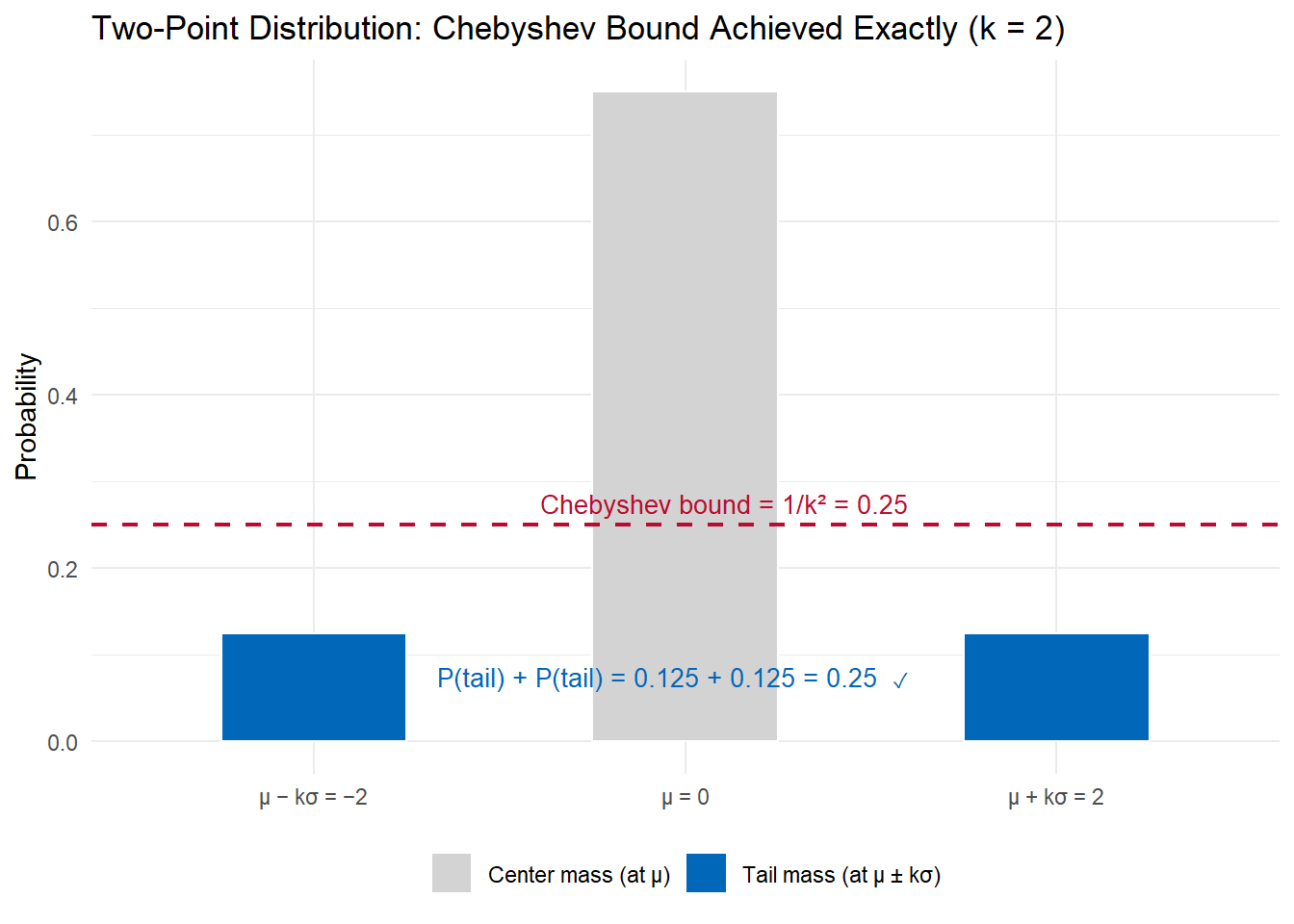
The total tail probability — the two blue bars — equals exactly \(\frac{1}{k^2} = 0.25\), touching the Chebyshev bound. This is the worst-case distribution for Chebyshev: any other distribution with the same mean and variance will have less tail probability beyond \(k\sigma\). Chebyshev’s bound cannot be improved in general because this distribution exists.
Let’s now see how the bound performs across several realistic distributions. All are standardized to \(\mu = 0\), \(\sigma = 1\) for direct comparison.
Now that we have Markov’s and Chebyshev’s inequalities, we can derive the Law of Large Numbers (LLN). It is one of the most fundamental results in probability and statistics, and it follows almost directly from Chebyshev.
Let \(X_1, X_2, \ldots, X_n\) be independent, identically distributed (i.i.d.) random variables with mean \(\mu\) and finite variance \(\sigma^2\). Define the sample mean:
\[\bar{X}_n = \frac{1}{n} \sum_{i=1}^n X_i\]
The Weak Law of Large Numbers states that for any \(\epsilon > 0\):
\[\lim_{n \to \infty} P\big(|\bar{X}_n - \mu| \geq \epsilon\big) = 0\]
As we collect more observations, the probability that the sample mean deviates from the true mean by any fixed amount \(\epsilon\) goes to zero. We say \(\bar{X}_n\) converges in probability to \(\mu\), written \(\bar{X}_n \xrightarrow{p} \mu\).
The derivation requires two preliminary results, then a direct application of Chebyshev’s Inequality.
Step 1: The expected value of \(\bar{X}_n\) is \(\mu\).
By linearity of expectation:
\[E[\bar{X}_n] = E\left[\frac{1}{n}\sum_{i=1}^n X_i\right] = \frac{1}{n}\sum_{i=1}^n E[X_i] = \frac{1}{n} \cdot n\mu = \mu\]
Step 2: The variance of \(\bar{X}_n\) is \(\sigma^2 / n\).
Because the \(X_i\) are independent, their variances add:
\[\text{Var}(\bar{X}_n) = \text{Var}\left(\frac{1}{n}\sum_{i=1}^n X_i\right) = \frac{1}{n^2}\sum_{i=1}^n \text{Var}(X_i) = \frac{1}{n^2} \cdot n\sigma^2 = \frac{\sigma^2}{n}\]
This is the key quantity: as \(n\) grows, the variance of the sample mean shrinks proportionally.
Step 3: Apply Chebyshev’s Inequality to \(\bar{X}_n\).
From Step 1, \(E[\bar{X}_n] = \mu\). From Step 2, \(\text{Var}(\bar{X}_n) = \sigma^2/n\). Chebyshev gives:
\[P\big(|\bar{X}_n - \mu| \geq \epsilon\big) \leq \frac{\text{Var}(\bar{X}_n)}{\epsilon^2} = \frac{\sigma^2}{n\epsilon^2}\]
Step 4: Take the limit.
For any fixed \(\epsilon > 0\) and \(\sigma^2 < \infty\):
\[\lim_{n \to \infty} P\big(|\bar{X}_n - \mu| \geq \epsilon\big) \leq \lim_{n \to \infty} \frac{\sigma^2}{n\epsilon^2} = 0\]
Since probabilities are non-negative, this forces \(P(|\bar{X}_n - \mu| \geq \epsilon) \to 0\). \(\square\)
Recap:
The variance of the sample mean is \(\sigma^2/n\) — it shrinks as observations accumulate. This is the engine of the result.
Chebyshev converts that shrinking variance into a shrinking probability bound. Without Chebyshev (or a similar inequality), we could not bridge from “variance → 0” to “probability of deviation → 0.”
The result holds for any distribution with finite mean and variance, regardless of shape. Normality is not required. The only assumption is \(\sigma^2 < \infty\).
Markov’s Inequality is the deeper foundation: Chebyshev was derived from Markov, so the LLN ultimately rests on Markov.
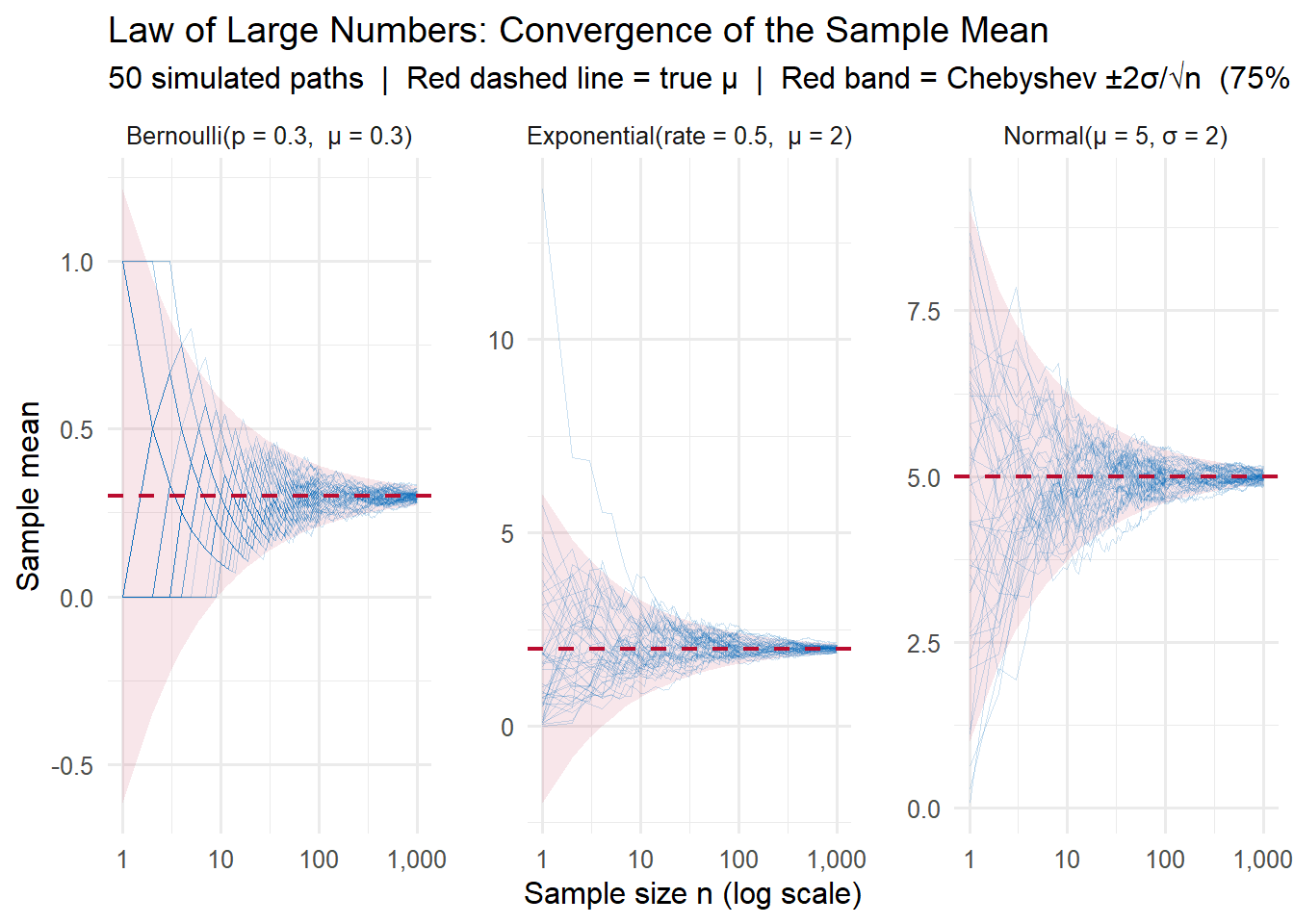
Let’s simulate the LLN across three distributions with very different shapes: a Normal, a skewed Exponential, and a discrete Bernoulli. This demonstrates that convergence holds regardless of the underlying distribution.
set.seed(4817)

n_obs  <- 1000  # maximum sample size
n_reps <- 50    # independent replications per distribution

# Each distribution with its natural mu and sigma
dist_params <- list(
  "Normal"      = list(mu = 5,   sigma = 2,               gen = function(n) rnorm(n, 5, 2)),
  "Exponential" = list(mu = 2,   sigma = 2,               gen = function(n) rexp(n, rate = 0.5)),
  "Bernoulli"   = list(mu = 0.3, sigma = sqrt(0.3 * 0.7), gen = function(n) rbinom(n, 1, 0.3))
)

# Simulate running (cumulative) means for all distributions
sim_data <- map_dfr(names(dist_params), function(d) {
  params  <- dist_params[[d]]
  X       <- matrix(params$gen(n_obs * n_reps), nrow = n_reps)
  running <- t(apply(X, 1, function(x) cumsum(x) / seq_along(x)))
  tibble(
    dist = d,
    rep  = rep(1:n_reps, each = n_obs),
    n    = rep(1:n_obs,  times = n_reps),
    xbar = as.vector(t(running))
  )
})

# Chebyshev ±2σ/√n envelope: P(|X̄ − μ| ≥ 2σ/√n) ≤ 1/4
band_data <- map_dfr(names(dist_params), function(d) {
  params <- dist_params[[d]]
  tibble(
    dist = d,
    n    = 1:n_obs,
    lo   = params$mu - 2 * params$sigma / sqrt(1:n_obs),
    hi   = params$mu + 2 * params$sigma / sqrt(1:n_obs)
  )
})
Plot 1: Running means converging to \(\mu\)
Each blue line is one simulated replication of \(\bar{X}_n\) as \(n\) grows. The red band is the Chebyshev \(\pm 2\sigma/\sqrt{n}\) envelope, within which at least 75% of paths must fall at every \(n\).
Plot 2: Chebyshev bound vs empirical violation rate
A direct check of the inequality from Step 3 of the derivation. At each \(n\), we measure what fraction of the 50 paths fall outside \(\epsilon = 0.5\sigma\) of \(\mu\) (blue), and compare to the theoretical bound \(\frac{\sigma^2}{n\epsilon^2}\) (red dashed). The bound holds everywhere, and both go to zero.
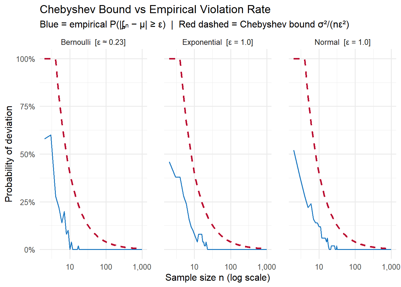
The Chebyshev bound (red) is conservative — as we saw in Section 2.2, Chebyshev’s bounds are loose for well-behaved distributions like the Normal. But the bound is guaranteed to hold for any distribution, and it is tight enough to prove the LLN: both the bound and the actual violation rate go to zero as \(n \to \infty\).
Markov’s Inequality gives a bound based on the mean. Chebyshev tightens it using the variance. Chernoff bounds go further, using the full moment generating function (MGF), and produce exponentially decaying tail probabilities rather than the polynomial \(1/k^2\) of Chebyshev.
Chernoff bounds are particularly useful for sums of independent random variables. For \(S_n = X_1 + \cdots + X_n\) with \(X_i \sim \text{Bernoulli}(p)\) and \(\mu = np\), the Chernoff bound states that for \(0 < \delta \leq 1\):
\[P(S_n \geq (1+\delta)\mu) \leq e^{-\mu\delta^2/3}\]
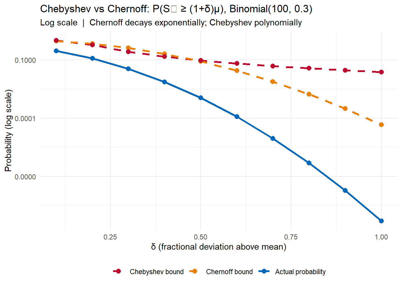
The key feature: the right-hand side decays exponentially in \(\mu\delta^2\). Compare this to Chebyshev’s \(\frac{1}{\delta^2}\), which decays only polynomially in \(\delta\).
Let’s see this in practice with \(S_n \sim \text{Binomial}(100, 0.3)\), so \(\mu = 30\).
n <- 100; p <- 0.3; mu <- n * p

delta_vals <- seq(0.1, 1.0, by = 0.1)
a_vals     <- (1 + delta_vals) * mu

bounds_df <- tibble(
  delta     = delta_vals,
  a         = a_vals,
  actual    = pbinom(a_vals - 1, n, p, lower.tail = FALSE),
  chernoff  = exp(-mu * delta_vals^2 / 3),
  chebyshev = pmin(1, (n * p * (1-p)) / (a_vals - mu)^2)
)

bounds_df |>
  mutate(across(actual:chebyshev, ~round(., 4))) |>
  flextable()
delta | a | actual | chernoff | chebyshev |
|---|---|---|---|---|
0.1 | 33 | 0.2893 | 0.9048 | 1.0000 |
0.2 | 36 | 0.1161 | 0.6703 | 0.5833 |
0.3 | 39 | 0.0340 | 0.4066 | 0.2593 |
0.4 | 42 | 0.0072 | 0.2019 | 0.1458 |
0.5 | 45 | 0.0011 | 0.0821 | 0.0933 |
0.6 | 48 | 0.0001 | 0.0273 | 0.0648 |
0.7 | 51 | 0.0000 | 0.0074 | 0.0476 |
0.8 | 54 | 0.0000 | 0.0017 | 0.0365 |
0.9 | 57 | 0.0000 | 0.0003 | 0.0288 |
1.0 | 60 | 0.0000 | 0.0000 | 0.0233 |
The Chernoff bound overtakes Chebyshev quickly. By \(\delta = 0.5\) (\(a = 45\)), Chebyshev says the probability is at most 9.3%, while Chernoff says at most 0.8%. The actual probability is 0.1%.
The derivation rests on a single idea: \(e^{tX}\) is a non-negative random variable, so Markov’s Inequality applies to it.
Step 1: Apply Markov to \(e^{tX}\).
For any \(t > 0\) and threshold \(a\):
\[P(X \geq a) = P\big(e^{tX} \geq e^{ta}\big) \leq \frac{E\big[e^{tX}\big]}{e^{ta}} = e^{-ta} \cdot M_X(t)\]
where \(M_X(t) = E[e^{tX}]\) is the moment generating function. This is valid for any \(t > 0\) because \(e^{tX}\) is non-negative.
Step 2: Optimize over \(t\).
Since the bound holds for all \(t > 0\), we take the minimum:
\[P(X \geq a) \leq \inf_{t > 0} \; e^{-ta} \cdot M_X(t)\]
Step 3: Apply to sums of independent variables.
For \(S_n = \sum_{i=1}^n X_i\) with \(X_i\) independent:
\[M_{S_n}(t) = \prod_{i=1}^n M_{X_i}(t) = M_X(t)^n\]
So the bound becomes \(e^{-ta} M_X(t)^n\), and we optimize over \(t > 0\).
Step 4: Specialize to Bernoulli.
For \(X_i \sim \text{Bernoulli}(p)\): \(M_X(t) = 1 - p + pe^t \leq e^{p(e^t - 1)}\).
With \(a = (1+\delta)\mu\) and \(\mu = np\), substituting and optimizing over \(t\) (setting \(t = \ln(1+\delta)\)):
\[P(S_n \geq (1+\delta)\mu) \leq \left(\frac{e^\delta}{(1+\delta)^{1+\delta}}\right)^\mu\]
Using the bound \((1+\delta)^{1+\delta} \geq e^{\delta + \delta^2/3}\) for \(0 < \delta \leq 1\) gives the simplified form:
\[P(S_n \geq (1+\delta)\mu) \leq e^{-\mu\delta^2/3}\]
Recap:
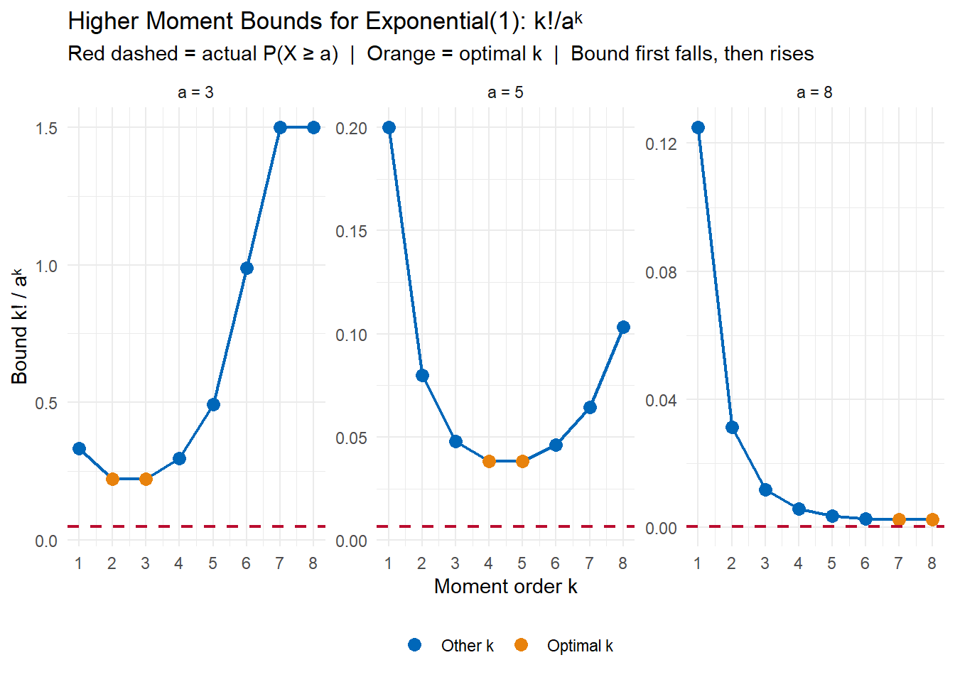
Markov uses the first moment. Chebyshev uses the second. A natural generalization: for any integer \(k \geq 1\) and non-negative random variable \(X\):
\[P(X \geq a) = P(X^k \geq a^k) \leq \frac{E[X^k]}{a^k}\]
Using higher moments tightens the bound when those moments are well-controlled. For the same threshold \(a\), a larger \(k\) can produce a smaller bound — provided \(E[X^k]\) doesn’t grow too fast.
Let’s apply this to \(X \sim \text{Exponential}(1)\), where \(E[X^k] = k!\) The actual tail probability is \(P(X \geq a) = e^{-a}\).
hm_df <- expand_grid(a = c(2, 3, 5, 8), k = 1:8) |>
  mutate(
    bound  = factorial(k) / a^k,
    actual = exp(-a),
    bound_capped = pmin(bound, 1)
  )

hm_df |>
  select(a, k, bound_capped, actual) |>
  mutate(across(c(bound_capped, actual), ~round(., 4))) |>
  pivot_wider(names_from = a, values_from = bound_capped,
              names_prefix = "a=") |>
  flextable() |>
  add_header_row(values = c("", "Bound k!/aᵏ  (actual probability in parentheses)"),
                 colwidths = c(2, 4))
Bound k!/aᵏ (actual probability in parentheses) | |||||
|---|---|---|---|---|---|
k | actual | a=2 | a=3 | a=5 | a=8 |
1 | 0.1353 | 0.50 | |||
2 | 0.1353 | 0.50 | |||
3 | 0.1353 | 0.75 | |||
4 | 0.1353 | 1.00 | |||
5 | 0.1353 | 1.00 | |||
6 | 0.1353 | 1.00 | |||
7 | 0.1353 | 1.00 | |||
8 | 0.1353 | 1.00 | |||
1 | 0.0498 | 0.333 | |||
2 | 0.0498 | 0.222 | |||
3 | 0.0498 | 0.222 | |||
4 | 0.0498 | 0.296 | |||
5 | 0.0498 | 0.494 | |||
6 | 0.0498 | 0.988 | |||
7 | 0.0498 | 1.000 | |||
8 | 0.0498 | 1.000 | |||
1 | 0.0067 | 0.2000 | |||
2 | 0.0067 | 0.0800 | |||
3 | 0.0067 | 0.0480 | |||
4 | 0.0067 | 0.0384 | |||
5 | 0.0067 | 0.0384 | |||
6 | 0.0067 | 0.0461 | |||
7 | 0.0067 | 0.0645 | |||
8 | 0.0067 | 0.1032 | |||
1 | 0.0003 | 0.1250 | |||
2 | 0.0003 | 0.0312 | |||
3 | 0.0003 | 0.0117 | |||
4 | 0.0003 | 0.0059 | |||
5 | 0.0003 | 0.0037 | |||
6 | 0.0003 | 0.0027 | |||
7 | 0.0003 | 0.0024 | |||
8 | 0.0003 | 0.0024 | |||
The optimal \(k\) — the one minimizing the bound — shifts to larger values as \(a\) grows. But even at the optimal \(k\), the bound remains considerably above the actual tail probability \(e^{-a}\). This shows a limitation of the moment approach: the factorial growth of \(k!\) causes the bound to eventually worsen for any fixed \(a\).
The derivation is a direct application of Markov’s Inequality.
For any non-negative random variable \(X\), raising both sides to the power \(k\) preserves the inequality:
\[X \geq a \implies X^k \geq a^k\]
So the two events are equivalent, and \(X^k\) is non-negative:
\[P(X \geq a) = P(X^k \geq a^k) \leq \frac{E[X^k]}{a^k}\]
This is it. The only question is which \(k\) gives the tightest bound, and that depends on how fast \(E[X^k]\) grows relative to \(a^k\). The connection to Chernoff is immediate: the Chernoff bound can be seen as applying this idea to the “continuous” analogue \(g(X) = e^{tX}\), which happens to grow more slowly (for the right distributions) than polynomial moments.
In high-dimensional space, something geometrically surprising happens. Draw a point uniformly at random from a \(d\)-dimensional standard Gaussian — that is, \(X = (X_1, \ldots, X_d)\) with each \(X_i \sim N(0,1)\) independently. Where does the point land?
In \(d = 2\) or \(d = 3\) dimensions, the mass is spread through the interior of a ball. But as \(d\) grows, the mass concentrates in a thin shell — an annulus — near the surface of a sphere of radius \(\sqrt{d}\). The interior of the ball is essentially empty.
The Gaussian Annulus Theorem makes this precise. For any \(\beta > 0\):
\[P\Big(|\, |X| - \sqrt{d}\,| \geq \beta\Big) \leq \frac{2}{\beta^2}\]
With probability at least \(1 - 2/\beta^2\), the norm \(|X|\) lies within \(\beta\) of \(\sqrt{d}\). The shell has width \(O(1)\) while its radius grows as \(\sqrt{d}\) — so the shell becomes relatively thinner as dimension increases.
Let \(Y = |X|^2 = \sum_{i=1}^d X_i^2\). We analyze \(Y\) first, then convert to a statement about \(|X|\).
Step 1: Mean and variance of \(Y\).
Each \(X_i^2\) has \(E[X_i^2] = 1\) and \(E[X_i^4] = 3\) (the fourth moment of the standard normal), so \(\text{Var}(X_i^2) = 3 - 1 = 2\). By independence:
\[E[Y] = d \qquad \text{Var}(Y) = 2d\]
Step 2: Apply Chebyshev to \(Y\).
\[P\big(|Y - d| \geq t\big) \leq \frac{\text{Var}(Y)}{t^2} = \frac{2d}{t^2}\]
Setting \(t = 2\beta\sqrt{d}\):
\[P\big(|\,|X|^2 - d\,| \geq 2\beta\sqrt{d}\big) \leq \frac{2d}{4\beta^2 d} = \frac{1}{2\beta^2}\]
Step 3: Convert from \(|X|^2\) to \(|X|\).
If \(|X|^2\) is within \(2\beta\sqrt{d}\) of \(d\), then \(|X|^2 \in [d - 2\beta\sqrt{d},\; d + 2\beta\sqrt{d}]\).
For large \(d\), \(2\beta\sqrt{d}\) is small relative to \(d\), so we can linearize: \(\sqrt{d \pm 2\beta\sqrt{d}} \approx \sqrt{d} \pm \beta\). Therefore \(|X| \in [\sqrt{d} - \beta,\; \sqrt{d} + \beta]\) with probability at least \(1 - 1/(2\beta^2)\).
A tighter statement using both tails gives the result:
\[P\Big(|\,|X| - \sqrt{d}\,| \geq \beta\Big) \leq \frac{2}{\beta^2}\]
Recap:
set.seed(3291)

n_samp <- 2000
d_vals <- c(2, 5, 20, 100, 500)

annulus_df <- map_dfr(d_vals, function(d) {
  X     <- matrix(rnorm(n_samp * d), nrow = n_samp)
  norms <- sqrt(rowSums(X^2))
  tibble(d = d, norm = norms, norm_scaled = norms / sqrt(d))
})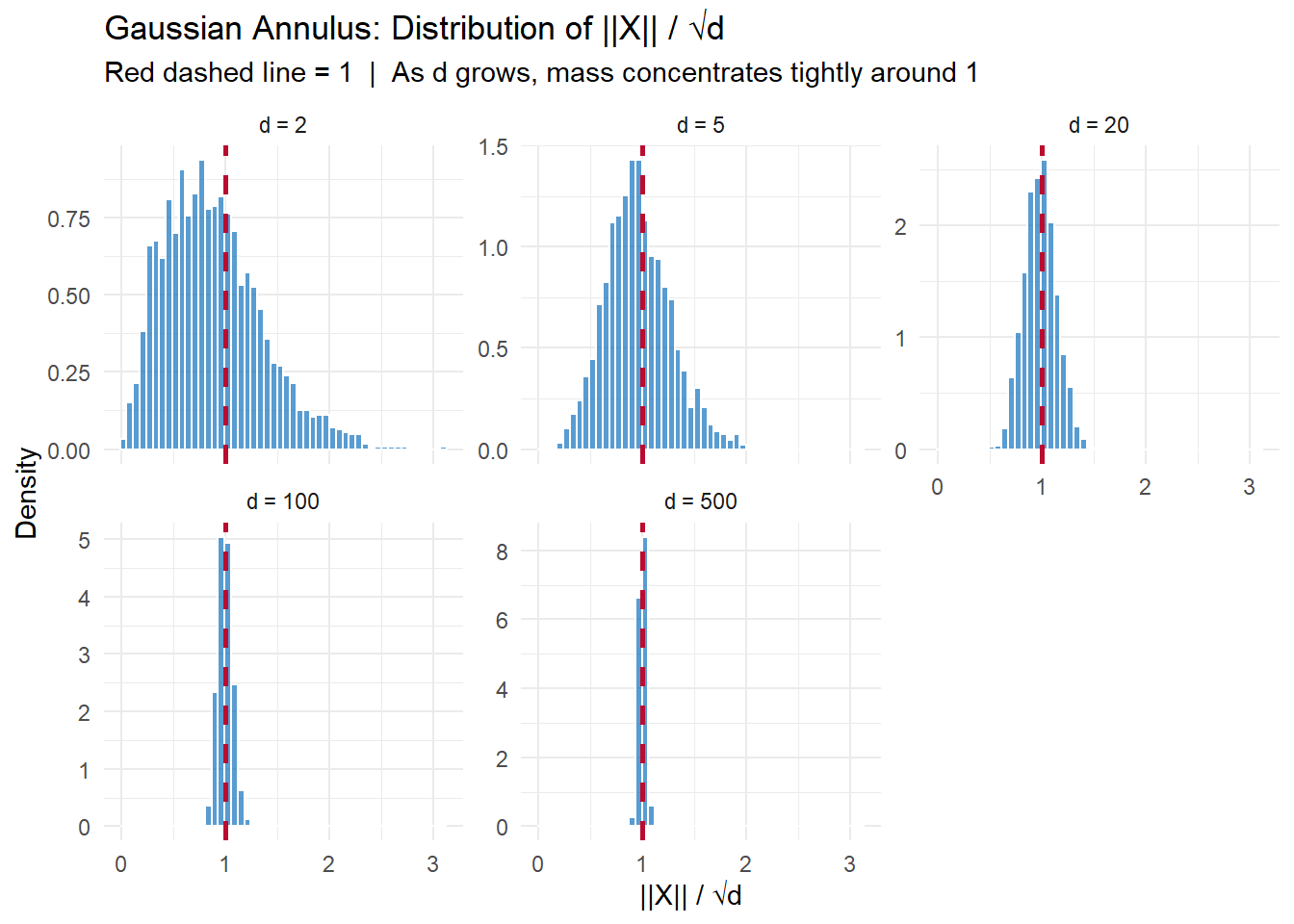
The spread of \(\|X\|/\sqrt{d}\) matches the theoretical standard deviation of \(1/\sqrt{2d}\) precisely:
annulus_df |>
  group_by(d) |>
  summarise(
    mean_norm_scaled = round(mean(norm_scaled), 4),
    sd_norm_scaled   = round(sd(norm_scaled), 4),
    theoretical_sd   = round(1 / sqrt(2 * d[1]), 4),
    .groups = "drop"
  ) |>
  flextable()
d | mean_norm_scaled | sd_norm_scaled | theoretical_sd |
|---|---|---|---|
2 | 0.883 | 0.4666 | 0.5000 |
5 | 0.957 | 0.3146 | 0.3162 |
20 | 0.989 | 0.1544 | 0.1581 |
100 | 0.998 | 0.0702 | 0.0707 |
500 | 1.000 | 0.0314 | 0.0316 |
As \(d\) increases from 2 to 500, the standard deviation of \(\|X\|/\sqrt{d}\) shrinks from 0.47 to 0.03 — following \(1/\sqrt{2d}\) closely. By \(d = 500\), virtually all points fall within 0.1 of the sphere of radius \(\sqrt{d}\).
A distribution follows a power law if its tail probability decays as a power of \(x\):
\[P(X \geq x) \sim C x^{-\alpha} \quad \text{for large } x\]
where \(\alpha > 0\) is the tail exponent. The smaller \(\alpha\), the heavier the tail.
Power laws arise in a wide range of phenomena: wealth (Pareto principle), city populations (Zipf’s law), earthquake magnitudes, degree distributions in networks, and insurance losses.
The Pareto distribution is the canonical example: for \(x \geq x_m\),
\[P(X \geq x) = \left(\frac{x_m}{x}\right)^\alpha\]
The moments of a Pareto distribution exist only up to order \(\alpha\):
| \(\alpha\) | Moments that exist | Implications |
|---|---|---|
| \(\alpha > 2\) | Mean and variance | Chebyshev applies; LLN holds normally |
| \(1 < \alpha \leq 2\) | Mean, but no variance | Chebyshev inapplicable; LLN holds, but convergence is slow |
| \(\alpha \leq 1\) | Neither mean nor variance | LLN breaks down entirely |
This is why power laws are problematic for standard statistical machinery: most of the inequalities derived in this chapter require at minimum a finite mean, and often a finite variance.
set.seed(7162)

rpareto <- function(n, alpha, x_m = 1) x_m / runif(n)^(1 / alpha)

n_obs_pl  <- 2000
n_reps_pl <- 30
alpha_vals <- c(0.8, 1.5, 2.5)

power_law_data <- map_dfr(alpha_vals, function(a) {
  mu_true <- if (a > 1) a / (a - 1) else NA_real_
  X       <- matrix(rpareto(n_obs_pl * n_reps_pl, a), nrow = n_reps_pl)
  running <- t(apply(X, 1, function(x) cumsum(x) / seq_along(x)))
  tibble(
    alpha   = a,
    rep     = rep(1:n_reps_pl, each = n_obs_pl),
    n       = rep(1:n_obs_pl,  times = n_reps_pl),
    xbar    = as.vector(t(running)),
    mu_true = mu_true
  )
})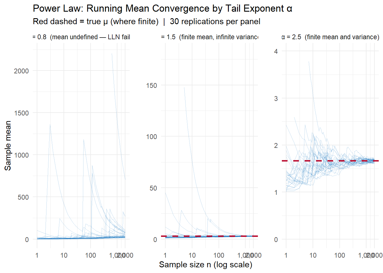
For \(\alpha = 2.5\): convergence is fast and tight, consistent with Chebyshev’s \(\sigma^2/n\) guarantee. For \(\alpha = 1.5\): the mean is finite (\(\mu = 3\)) and the sample mean does converge, but slowly and erratically — the infinite variance means Chebyshev gives no useful bound. For \(\alpha = 0.8\): there is no finite mean to converge to. The running means wander without settling, and the occasional enormous draw can shift the average dramatically even at large \(n\).
All of the concentration inequalities in this chapter follow from a single idea. For any non-decreasing function \(g \geq 0\):
\[P(X \geq a) = P\big(g(X) \geq g(a)\big) \leq \frac{E\big[g(X)\big]}{g(a)}\]
The first equality holds because \(g\) is non-decreasing. The inequality is Markov’s Inequality applied to the non-negative random variable \(g(X)\).
Every result in this chapter is a special case of this template:
| Bound | Choice of \(g(x)\) | Resulting bound |
|---|---|---|
| Markov | \(g(x) = x\) | \(E[X]\;/\;a\) |
| Chebyshev | \(g(x) = (x - \mu)^2\) | \(\text{Var}(X)\;/\;\epsilon^2\) |
| \(k\)-th moment | \(g(x) = x^k\) | \(E[X^k]\;/\;a^k\) |
| Chernoff | \(g(x) = e^{tx}\) | \(e^{-ta}\,M_X(t)\) |
The “art” in applying the master theorem is choosing \(g\) to minimize the resulting bound for the distribution and threshold at hand. The choices above are not arbitrary:
The Chernoff bound is so powerful because \(e^{tx}\) amplifies large values of \(X\) more aggressively than any polynomial. When \(X\) is unlikely to be large, this aggressive amplification means \(E[e^{tX}]\) remains small, and the bound is tight.
Bound | g(x) | Value | Actual |
|---|---|---|---|
Markov | x | 0.333 | 0.0498 |
Chebyshev (k=2) | (x − μ)² | 0.222 | 0.0498 |
4th Moment | x⁴ | 0.296 | 0.0498 |
Chernoff | eᵗˣ | 0.406 | 0.0498 |
For \(X \sim \text{Exponential}(1)\) at \(a = 3\): Markov gives 0.333, Chebyshev gives 0.222, the 4th moment gives 0.296, and Chernoff gives 0.100 — against an actual probability of 0.050. Each tighter bound requires more information about the distribution (mean → variance → higher moments → full MGF), but rewards that information with a smaller bound.